This example will use the tips dataset, which records the tips a waiter got over a period of a couple months. In a previous example we found that tips was rather skewed, so we will also examine log(tips).
Enter the following into the console:
data(tips)
tips$log_tip<-log(tips$tip)
tips$tip_percentage<-100*tips$tip/tips$total_bill
Variables:
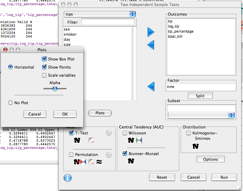
We will examine the differences in tip, log_tip, tip_percentage and total_bill by entering them as outcomes. The factor is time. We will perform two types of tests on these variables, the t-test, and the brunner-munzel test (which is resistant to outliers). Additionally we will obtain unscaled plots by deselecting 'Scaled Variables"
descriptive.table(d(tip,log_tip,tip_percentage,total_bill),time,tips,func.names =c("Mean","St. Deviation","Valid N"))
print(two.sample.test(formula=d(tip,log_tip,tip_percentage,total_bill) ~ time,
		data=tips,
		test=t.test,
		alternative="two.sided")
)
library(lawstat)
print(two.sample.test(formula=d(tip,log_tip,tip_percentage,total_bill) ~ time,
		data=tips,
		test=brunner.munzel.test,
		alternative="two.sided")
)
oneway.plot(formula=d(tip,log_tip,tip_percentage,total_bill)~time,data=tips,
	alpha=0.51))
> descriptive.table(d(tip,log_tip,tip_percentage,total_bill),time,tips,func.names =c("Mean","St. Deviation","Valid N"))
$`strata: Dinner `
                    Mean St. Deviation Valid N
tip             3.102670     1.4362428     176
log_tip         1.034377     0.4462253     176
tip_percentage 15.951779     6.7477139     176
total_bill     20.797159     9.1420292     176

$`strata: Lunch `
                     Mean St. Deviation Valid N
tip             2.7280882     1.2053454      68
log_tip         0.9201313     0.4004058      68
tip_percentage 16.4127928     4.0241549      68
total_bill     17.1686765     7.7138818      68

> print(two.sample.test(formula=d(tip,log_tip,tip_percentage,total_bill) ~ time,
+ data=tips,
+ test=t.test,
+ alternative="two.sided")
+ )
                                            Welch Two Sample t-test
               mean of Dinner mean of Lunch Difference 95% CI Lower 95% CI Upper          t       df
tip                  3.102670     2.7280882  0.3745822  0.015053640    0.7341108  2.0593266 144.0712
log_tip              1.034377     0.9201313  0.1142453 -0.002574869    0.2310655  1.9341221 134.8400
tip_percentage      15.951779    16.4127928 -0.4610139 -1.850914865    0.9288870 -0.6540376 200.8764
total_bill          20.797159    17.1686765  3.6284826  1.331876787    5.9250885  3.1229862 143.2927
                   p-value
tip            0.041263422
log_tip        0.055192775
tip_percentage 0.513835616
total_bill     0.002166574
  HA: two.sided
  H0:  difference in means = 0
> library(lawstat)
> print(two.sample.test(formula=d(tip,log_tip,tip_percentage,total_bill) ~ time,
+ data=tips,
+ test=brunner.munzel.test,
+ alternative="two.sided")
+ )
                                              Brunner-Munzel Test
               P(X<Y)+.5*P(X=Y) 95% CI Lower 95% CI Upper Brunner-Munzel Test Statistic       df      p-value
tip                   0.4098429    0.3294411    0.4902447                     -2.219022 126.3503 0.0282701762
log_tip               0.4098429    0.3294411    0.4902447                     -2.219022 126.3503 0.0282701762
tip_percentage        0.5495906    0.4718788    0.6273023                      1.260831 150.9286 0.2093154159
total_bill            0.3660177    0.2877780    0.4442575                     -3.389074 125.3488 0.0009379292
> oneway.plot(formula=d(tip,log_tip,tip_percentage,total_bill)~time,data=tips,
+ alpha=0.51)
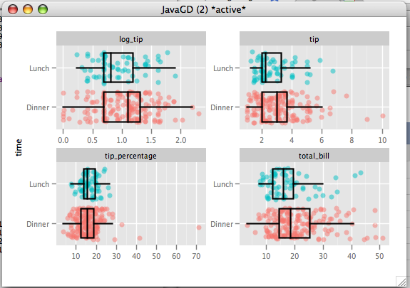
We can see from the plot that tip and total_bill are skewed, and tip_percentage has a number of large outliers (one party tipped 70%!!). We have a sample size of 244, which is fairly large, so we don't have to worry to much about the normality assumption. That said, due to their skew, comparing the means (as a t-test does) may not be the best method. The outliers in tip_percentage indicate that we should go with a robust method, at least for tip_percentage.
The brunner-munzel test, which compares central tendency (not means) and is robust to outliers, shows significance for tip (p=.028), log_tip(p=.028), and total_bill(p<.001). tip_percentage on the other hand is not significant (p=.209). From this we can conclude that dinner parties do tip more, and they have larger bills. They are not detectably more generous than the lunch customers because they tip a similar percentage of the bill.
 Deducer: A GUI for R